Squares? What squares? Show me the squares!
This is an illustration of the “Least Squares” method. These are the “squares” that you’ve been hearing about all along. Johann Carl Friedrich Gauss proved that it’s enough for most of the things we observe on Earth and in Universe.
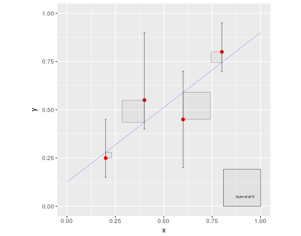
This picture shows squares of the distance from the ‘experimental points’ to the line. In order to visualize the function dist^2 we have drawn the areas proportional to these distances as squares. The sum of these areas (the gray square in the lower right corner) depends on the way you draw the line between the points. If you are like me (and many other people) and can in your mind imagine the parts of the picture moving, you immediately get an idea of how the whole method works. If you (in your imagination) start moving or tilting the line, the squares (and their area) will be changing in a certain way. The name of the game is to make the sum of all their areas as small as possible. Remember that the bigger the side of the square already is - the faster its area changes if you increase it a bit (and the faster it decreases if you make the side of the square smaller)… Just play with this picture in your mind for a little while. I wish somebody would have shown it to me when I was 10 years old and I would be able to do it then.
… if you can not do it in your head, never mind, here’s the illustration for you.
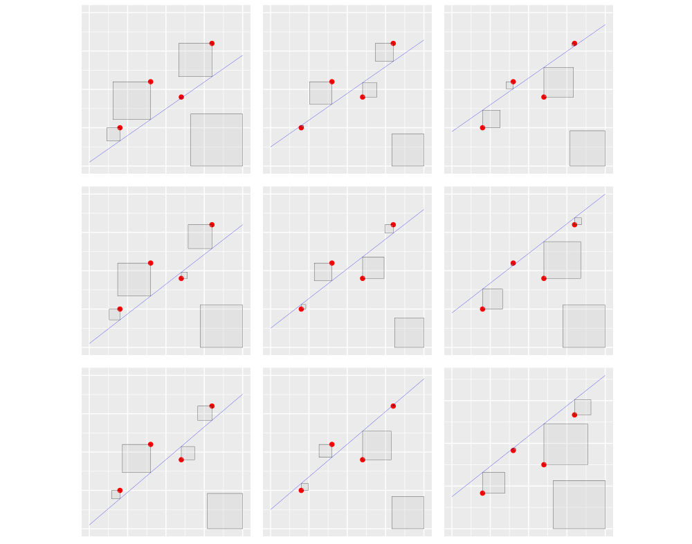
The optimized picture is in the middle, the pictures with variations of parameters are around it (different offsets are in different columns, different slopes are in different rows).
More about these pictures and how to draw them and similar ones in R Illustration for the Least Squares Method repo .